Thursday, March 24, 2022

Spark Checkpointing vs Persist

 Checkpointing saves an RDD to a reliable storage system (e.g. HDFS, S3) while forgetting the RDD's lineage completely.  As the driver restarts the recovery takes place.

There are two types of data that we checkpoint in Spark:

Metadata Checkpointing – Metadata means the data about data. It refers to saving the metadata to fault tolerant storage like HDFS. Metadata includes configurations, DStream operations, and incomplete batches. Configuration refers to the configuration used to create streaming DStream operations are operations which define the steaming application. Incomplete batches are batches which are in the queue but are not complete.

Data Checkpointing –: It refers to save the RDD to reliable storage because its need arises in some of the stateful transformations. It is in the case when the upcoming RDD depends on the RDDs of previous batches. Because of this, the dependency keeps on increasing with time. Thus, to avoid such increase in recovery time the intermediate RDDs are periodically checkpointed to some reliable storage. As a result, it cuts down the dependency chain.

To set the Spark checkpoint directory call: SparkContext.setCheckpointDir(directory: String)

3. Types of Checkpointing in Apache Spark

There are two types of Apache Spark checkpointing:

Reliable Checkpointing – It refers to that checkpointing in which the actual RDD is saved in reliable distributed file system, e.g. HDFS. To set the checkpoint directory call: SparkContext.setCheckpointDir(directory: String). When running on the cluster the directory must be an HDFS path since the driver tries to recover the checkpointed RDD from a local file. While the checkpoint files are actually on the executor’s machines.

Local Checkpointing: In this checkpointing, in Spark Streaming or GraphX we truncate the RDD lineage graph in Spark. In this, the RDD is persisted to local storage in the executor.

Apache Spark Quiz

Difference between Spark Checkpointing and Persist


                  Checkpointing

                          Persist

Checkpointing stores the RDD in HDFS. It deletes the lineage which created it.

When we persist RDD with DISK_ONLY storage level the RDD gets stored in a location where the subsequent use of that RDD will not reach that point in recomputing the lineage.

On completing the job run unlike cache the checkpoint file is not deleted.

When we are checkpointing an RDD it results in double computation. The operation will first call a cache before accomplishing the actual job of computing. Secondly, it is written to checkpointing directory.

After persist() is called, Spark remembers the lineage of the RDD even though it doesn’t call it.

Secondly, after the job run is complete, the cache is cleared and the files are destroyed.

Checkpointing is reliable.

Persisting is unreliable.

Difference between executor and container in Spark

  •  Spark Executor runs within a Yarn Container, not across Containers.
  • A Yarn Container is provided by the YARN Resource Manager on demand - at start of Spark Application of via YARN Dynamic Resource Allocation.
  • A Yarn Container can have only one Spark Executor, but 1 or indeed more Cores can be assigned to the Executor.
  • Each Spark Executor and Driver runs as part of its own YARN Container.
  • Executors run on a given Worker.
  • Moreover, everything is in the context of an Application and as such an Application has Executors on many Workers.

Spark Application - Troubleshooting Stragglers (slow executing tasks)


Stragglers in your Spark Application affect the overall application performance and waste premium resources.

Stragglers are detrimental to the overall performance of Spark applications and lead to resource wastages on the underlying cluster. Therefore, it is important to identify potential stragglers in your Spark Job, identify the root cause behind them, and put required fixes or provide preventive measures.

A straggler refers to a very very slow executing Task belonging to a particular stage of a Spark application (Every stage in Spark is composed of one or more Tasks, each one computing a single partition out of the total partitions designated for the stage). A straggler Task takes an exceptionally high time for completion as compared to the median or average time taken by other tasks belonging to the same stage. There could be multiple stragglers in a Spark Job being present either in the same stage or across multiple stages.

Even if one straggler is present in a Spark stage, it would considerably delay the execution of the stage with its presence. Delayed execution of one or more stages (due to stragglers), in turn, would have a domino effect on the overall execution performance of the Spark App.

Further, stragglers could also lead to wastage of cluster resources if static resources are configured for the Job. This is due to the fact that unless the stragglers are finished, the already freed static resources of the stage can’t be put to use in the future stages that are dependent on the straggler affected stage.

The presence of stragglers can be felt when you observe that a stage progress bar (available in the Spark UI) corresponding to an executed stage gets stuck in the end. To confirm the same, you could open the stage-specific details listing the summary of Task metrics of completed tasks in the stage. If the Task metric shows that ‘Max duration’ among the completed tasks is exceptionally higher than the ‘Median’ or ‘75th percentile’ value, then it indicates the possibility of stragglers in the corresponding Job. Here is an example showing Task metrics snapshot of a straggler inflicted stage of a Job:

In the above snapshot, it is clearly evident that the corresponding stage suffered from the stragglers, as the ‘Max’ Task duration, which is 28 min, is exceptionally higher than the ‘75th percentile’ value which is only a meager 14 seconds. Further, the individual stragglers can be identified from the detailed Task description section of the stage-specific page. All those tasks whose execution duration lies above the ‘75th percentile’ value can be classified as stragglers for the stage.

: Here are some of the common reasons for stragglers problem:

Skewed partitioning: This is one of the widespread and the most common cause of stragglers. Skewed partitioning results in skewed partitions (skewness with respect to data size mapped to each of the partition). And, if the partition data directly reflects the data to be computed upon, then skewed partitions result in a skewed distribution of computation time among tasks assigned for them thereby giving birth to stragglers.

Skewed partitioning can arise in multiple scenarios, the most common being repartitioning of a Dataset or RDD on the basis of partitioning key having a skewed distribution.

Skewed partitioning could also result when a bunch of unsplittable files, skewed by the size, are read into a Dataset/RDD.

Skewed Computation: This is another widespread reason for giving rise to stragglers. If you are doing custom computation on partitions data, it may happen that the computation gets skewed among the partitions owning to dependence on certain attributes/properties of the data (residing in the partition) even though the data among partitions is distributed fairly well. Now, once the computation gets skewed, again it could potentially result in stragglers.

Imbalanced/Skewed computation can arise in scenarios where the computing work in the computing routine of the partition is directly proportional to certain properties of the data records in the partition. An example would be a case where a Dataset points to a collection of FileWrappers Objects, and in a particular partition of this Dataset, all corresponding FileWrapper Objects refer to relatively big files as compared to FileWrapper Objects residing in the other partitions. The particular partition in the example, therefore could give rise to a straggler task.

Slow disk reads/writes: Stragglers can potentially arise for stages, requiring disk read/writes when some of the corresponding tasks are hosted on a server that is suffering from slow disk read/writes.

Stages would involve disk read/writes when they require to execute a shuffle read/write operations or save an intermediate RDD/Dataset on to the disk.

Higher Number of Cores per Executor: Provisioning a higher number of cores per executor, in ranges such as 4~8, could also sometimes lead to potential stragglers. This may happen because of the possibility of simultaneous execution of compute/resource heavy tasks on all the cores of an executor. Simultaneous execution situation could lead to fighting for common resources, such as memory, within the hosting executor which could lead to performance deteriorating events, such as heavy garbage collection, which in turn could potentially give rise to stragglers in the stage.

:

Fair Partitioning: You need to ensure that the data is fairly partitioned among all the partitions when the computation intensity is directly related to the size of data contained in a partition. If there is flexibility in choosing a re-partitioning key, one should go for a record attribute, as a key, which provides higher cardinality and is evenly distributed among data records. If there is no such flexibility available, and the repartitioning key distribution is highly skewed, one can opt and try salting techniques.

Fair Computation: You also need to ensure that computation is evenly distributed among partitions where computation intensity is not directly related to the size of data in a partition but is dependent on the certain attribute or field in each of the data records.

Increased Number of Partitions: Increasing the number of partitions could decrease the magnitude of performance penalty afflicted by the stragglers. However, this would help to a certain extent only. ( To know more about the Spark partitioning tuning, you could refer to, “Guide to Spark Partitioning: Spark Partitioning Explained in Depth” )

Turning on the Spark speculation feature: Spark speculation feature, which actively identifies slow-running tasks, kills them and again re-launches the same, can optionally be turned on to deal with stragglers. It helps in dealing with stragglers that arise due to resource crunch on executors or due to slow disk/network read/writes on the hosting server. By default, the feature is turned off, one can enable the same by setting the spark config, spark. speculation’ to true. Further, the speculation feature provides various other knobs too (in terms of spark config) to fine-tune the straggler identification and killing behavior. Here is the description of these knobs:

a) spark.speculation.interval (default: 100ms): How often Spark will check for tasks to speculate. You need not touch the same.

b) spark.speculation.multiplier (default: 1.5): How many times slower a task is than the median to be considered for speculation. This is used as a criterion for identifying the stragglers and can be tuned based on Spark application behavior.

c) spark.speculation.quantile (default: 0.75): Fraction of tasks which must be complete before speculation is enabled for a particular stage. This is used to decide when to launch the attack and kill the stragglers and further re-launch them, this can also be tuned based on Spark application behavior.

Although speculation seems to be a readymade feature to address the straggler menace, try it only after you study your application behavior. Rather, I would advise you to first find the root cause for stragglers and provide fixes accordingly, because killing and re-launch of tasks, at times, could result in inconsistencies in application output.

Here is the Task metrics snapshot of the earlier example after the corresponding application is re-worked to address the straggler’s problem.

As you can be from the snapshot, the max time has now been reduced to 1.7 minutes from the earlier 28 minutes

Spark - Data Skew in UI

 Memory management and deals with issues that arise with data skew and garbage collection in Spark. Like many performance challenges with Spark, the symptoms increase as the scale of data handled by the application increases.

What is Data Skew?

In an ideal Spark application run, when Spark wants to perform a join, for example, join keys would be evenly distributed and each partition would get nicely organized to process. However, real business data is rarely so neat and cooperative. We often end up with less than ideal data organization across the Spark cluster that results in degraded performance due to data skew.

Data skew is not an issue with Spark per se, rather it is a data problem. The cause of the data skew problem is the uneven distribution of the underlying data. Uneven partitioning is sometimes unavoidable in the overall data layout or the nature of the query.

For joins and aggregations Spark needs to co-locate records of a single key in a single partition.  Records of a key will always be in a single partition. Similarly, other key records will be distributed in other partitions. If a single partition becomes very large it will cause data skew, which  will be problematic for any query engine if no special handling is done.

Dealing with data skew

Data skew problems are more apparent in situations where data needs to be shuffled in an operation such as a join or an aggregation. Shuffle is an operation done by Spark to keep related data (data pertaining to a single key) in a single partition. For this, Spark needs to move data around the cluster. Hence shuffle is considered the most costly operation.

Common symptoms of data skew are

  • Stuck stages & tasks
  • Low utilization of CPU
  • Out of memory errors

There are several tricks we can employ to deal with data skew problem in Spark. 

Identifying and resolving data skew

Spark users often observe all tasks finish within a reasonable amount of time, only to have one task take forever. In all likelihood, this is an indication that your dataset is skewed.  This behavior also results in the overall underutilization of the cluster. This is especially a problem when running Spark in the cloud, where over-provisioning of  cluster resources is wasteful and costly.

If skew is at the data source level (e.g. a hive table is partitioned on _month key and table has a lot more records for a particular _month),  this will cause skewed processing in the stage that is reading from the table. In such a case restructuring the table with a different partition key(s) helps. However, sometimes it is not feasible as the table might be used by other data pipelines in an enterprise.

In such cases, there are several things that we can do to avoid skewed data processing.

DATA BROADCAST

If we are doing a join operation on a skewed dataset one of the tricks is to increase the “spark.sql.autoBroadcastJoinThreshold” value so that smaller tables get broadcasted. This should be done to ensure sufficient driver and executor memory.

DATA PREPROCESS

If there are too many null values in a join or group-by key they would skew the operation. Try to preprocess the null values with some random ids and handle them in the application.

SALTING

In a SQL join operation, the join key is changed to redistribute data in an even manner so that processing for a partition does not take more time. This technique is called salting. Let’s take an example to check the outcome of salting. In a join or group-by operation, Spark maps a key to a particular partition id by computing a hash code on the key and dividing it by the number of shuffle partitions.

Let’s assume there are two tables with the following schema.

Let’s consider a case where a particular key is skewed heavily e.g. key 1, and we want to join both the tables and do a grouping to get a count. For example,

After the shuffle stage induced by the join operation, all the rows having the same key needs to be in the same partition. Look at the above diagram. Here all the rows of key 1 are in partition 1. Similarly, all the rows with key 2 are in partition 2. It is quite natural that processing partition 1 will take more time, as the partition contains more data. Let’s check Spark’s UI for shuffle stage run time for the above query.

As we can see one task took a lot more time than other tasks. With more data it would be even more significant. Also, this might cause application instability in terms of memory usage as one partition would be heavily loaded.

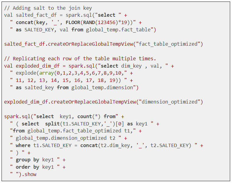
Can we add something to the data, so that our dataset will be more evenly distributed? Most of the users with skew problem use the salting technique. Salting is a technique where we will add random values to join key of one of the tables. In the other table, we need to replicate the rows to match the random keys.The idea is if the join condition is satisfied by key1 == key1, it should also get satisfied by key1_<salt> = key1_<salt>. The value of salt will help the dataset to be more evenly distributed.

Here is an example of how to do that in our use case. Check the number 20, used while doing a random function & while exploding the dataset. This is the distinct number of divisions we want for our skewed key. This is a very basic example and can be improved to include only keys which are skewed.

Now let’s check the Spark UI again. As we can see processing time is more even now

Note that for smaller data the performance difference won’t be very different. Sometimes the shuffle compress also plays a role in the overall runtime. For skewed data, shuffled data can be compressed heavily due to the repetitive nature of data. Hence the overall disk IO/ network transfer also reduces. We need to run our app without salt and with salt to finalize the approach that best fits our case.

Garbage Collection

Spark runs on the Java Virtual Machine (JVM). Because Spark can store large amounts of data in memory, it has a major reliance on Java’s memory management and garbage collection (GC). Therefore, garbage collection  (GC) can be a major issue that can affect many Spark applications.

Common symptoms of excessive GC in Spark are:

  • Slowness of application
  • Executor heartbeat timeout
  • GC overhead limit exceeded error

Spark’s memory-centric approach and data-intensive applications make it a more common issue than other Java applications. Thankfully, it’s easy to diagnose if your Spark application is suffering from a GC problem. The Spark UI marks executors in red if they have spent too much time doing GC.

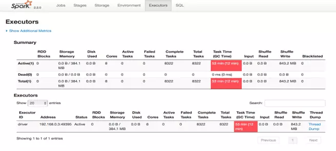
Spark executors are spending a significant amount of CPU cycles performing garbage collection. This can be determined by looking at the “Executors” tab in the Spark application UI. Spark will mark an executor in red if the executor has spent more than 10% of the time in garbage collection than the task time as you can see in the diagram below.

The Spark UI indicates excessive GC in red

Addressing garbage collection issues

Here are some of the basic things we can do to try to address GC issues.

DATA STRUCTURES

If using RDD based applications, use data structures with fewer objects. For example, use an array instead of a list. 

SPECIALIZED DATA STRUCTURES

If you are dealing with primitive data types, consider using specialized data structures like Koloboke or fastutil. These structures optimize memory usage for primitive types.

STORING DATA OFF-HEAP

The Spark execution engine and Spark storage can both store data off-heap. You can switch on off-heap storage using

  • –conf spark.memory.offHeap.enabled = true
  • –conf spark.memory.offHeap.size = Xgb.

Be careful when using off-heap storage as it does not impact on-heap memory size i.e. it won’t shrink heap memory. So to define an overall memory limit, assign a smaller heap size.

BUILT-IN VS USER DEFINED FUNCTIONS (UDFS)

If you are using Spark SQL, try to use the built-in functions as much as possible, rather than writing new UDFs. Most of the SPARK UDFs can work on UnsafeRow and don’t need to convert to wrapper data types. This avoids creating garbage, also it plays well with code generation.

BE STINGY ABOUT OBJECT CREATION

Remember we may be working with billions of rows. If we create even a small temporary object with 100-byte size for each row, it will create 1 billion * 100 bytes of garbage.

End of Part II

So far, we have focused on memory management, data skew and garbage collection as causes of slowdowns and failures in your Spark applications.

Spark Optimization Techniques

A Spark job can be optimized by many techniques so let’s dig deeper into those techniques one by one. Apache Spark optimization helps with in-memory data computations. The bottleneck for these spark optimization computations can be CPU, memory or any resource in the cluster. 1. Serialization Serialization plays an important role in the performance for any distributed application. By default, Spark uses Java serializer. Spark can also use another serializer called ‘Kryo’ serializer for better performance. Kryo serializer is in compact binary format and offers processing 10x faster than Java serializer. To set the serializer properties: conf.set(“spark.serializer”, “org.apache.spark.serializer.KryoSerializer”) Code: val conf = new SparkConf().setMaster(…).setAppName(…) conf.registerKryoClasses(Array(classOf[MyClass1], classOf[MyClass2])) val sc = new SparkContext(conf) Serialization plays an important role in the performance of any distributed application and we know that by default Spark uses the Java serializer on the JVM platform. Instead of Java serializer, Spark can also use another serializer called Kryo. The Kryo serializer gives better performance as compared to the Java serializer. Kryo serializer is in a compact binary format and offers approximately 10 times faster speed as compared to the Java Serializer. To set the Kryo serializer as part of a Spark job, we need to set a configuration property, which is org.apache.spark.serializer.KryoSerializer. 2. API selection Spark introduced three types of API to work upon – RDD, DataFrame, DataSet RDD is used for low level operation with less optimization DataFrame is best choice in most cases due to its catalyst optimizer and low garbage collection (GC) overhead. Dataset is highly type safe and use encoders. It uses Tungsten for serialization in binary format. We know that Spark comes with 3 types of API to work upon -RDD, DataFrame and DataSet. RDD is used for low-level operations and has less optimization techniques. DataFrame is the best choice in most cases because DataFrame uses the catalyst optimizer which creates a query plan resulting in better performance. DataFrame also generates low labor garbage collection overhead. DataSets are highly type safe and use the encoder as part of their serialization. It also uses Tungsten for the serializer in binary format. Code: val df = spark.read.json(“examples/src/main/resources/people.json”) case class Person(name: String, age: Long) // Encoders are created for case classes val caseClassDS = Seq(Person(“Andy”, 32)).toDS() // Encoders for most common types are automatically provided by importing spark.implicits._ val primitiveDS = Seq(1, 2, 3).toDS() primitiveDS.map(_ + 1).collect() // Returns: Array(2, 3, 4) // DataFrames can be converted to a Dataset by providing a class. Mapping will be done by name val path = “examples/src/main/resources/people.json” val peopleDS = spark.read.json(path).as[Person] 3. Advance Variable Broadcasting plays an important role while tuning Spark jobs. Broadcast variable will make small datasets available on nodes locally. When you have one dataset which is smaller than other dataset, Broadcast join is highly recommended. To use the Broadcast join: (df1. join(broadcast(df2))) Spark comes with 2 types of advanced variables – Broadcast and Accumulator. Broadcasting plays an important role while tuning your spark job. Broadcast variable will make your small data set available on each node, and that node and data will be treated locally for the process. Suppose you have a situation where one data set is very small and another data set is quite large, and you want to perform the join operation between these two. In that case, we should go for the broadcast join so that the small data set can fit into your broadcast variable. The syntax to use the broadcast variable is df1.join(broadcast(df2)). Here we have a second dataframe that is very small and we are keeping this data frame as a broadcast variable. Code: val broadcastVar = sc.broadcast(Array(1, 2, 3)) broadcastVar.value res0: Array[Int] = Array(1, 2, 3) val accum = sc.longAccumulator(“My Accumulator”) sc.parallelize(Array(1, 2, 3, 4)).foreach(x => accum.add(x)) accum.value res2: Long = 10 4. Cache and Persist Spark provides its own caching mechanisms like persist() and cache(). cache() and persist() will store the dataset in memory. When you have a small dataset which needs be used multiple times in your program, we cache that dataset. Cache() – Always in Memory Persist() – Memory and disks Spark provides its own caching mechanism like Persist and Caching. Persist and Cache mechanisms will store the data set into the memory whenever there is requirement, where you have a small data set and that data set is being used multiple times in your program. If we apply RDD.Cache() it will always store the data in memory, and if we apply RDD.Persist() then some part of data can be stored into the memory some can be stored on the disk. 5. ByKey Operation Shuffles are heavy operation which consume a lot of memory. While coding in Spark, the user should always try to avoid shuffle operation. High shuffling may give rise to an OutOfMemory Error; To avoid such an error, the user can increase the level of parallelism. Use reduceByKey instead of groupByKey. Partition the data correctly. As we know during our transformation of Spark we have many ByKey operations. ByKey operations generate lot of shuffle. Shuffles are heavy operation because they consume a lot of memory. While coding in Spark, a user should always try to avoid any shuffle operation because the shuffle operation will degrade the performance. If there is high shuffling then a user can get the error out of memory. Inthis case, to avoid that error, a user should increase the level of parallelism. Instead of groupBy, a user should go for the reduceByKey because groupByKey creates a lot of shuffling which hampers the performance, while reduceByKey does not shuffle the data as much. Therefore, reduceByKey is faster as compared to groupByKey. Whenever any ByKey operation is used, the user should partition the data correctly. 6. File Format selection Spark supports many formats, such as CSV, JSON, XML, PARQUET, ORC, AVRO, etc. Spark jobs can be optimized by choosing the parquet file with snappy compression which gives the high performance and best analysis. Parquet file is native to Spark which carries the metadata along with its footer. Spark comes with many file formats like CSV, JSON, XML, PARQUET, ORC, AVRO and more. A Spark job can be optimized by choosing the parquet file with snappy compression. Parquet file is native to Spark which carry the metadata along with its footer as we know parquet file is native to spark which is into the binary format and along with the data it also carry the footer it’s also carries the metadata and its footer so whenever you create any parquet file, you will see .metadata file on the same directory along with the data file. Code: val peopleDF = spark.read.json(“examples/src/main/resources/people.json”) peopleDF.write.parquet(“people.parquet”) val parquetFileDF = spark.read.parquet(“people.parquet”) val usersDF = spark.read.format(“avro”).load(“examples/src/main/resources/users.avro”) usersDF.select(“name”, “favorite_color”).write.format(“avro”).save(“namesAndFavColors.avro”) 7. Garbage Collection Tuning JVM garbage collection can be a problem when you have large collection of unused objects. The first step in GC tuning is to collect statistics by choosing – verbose while submitting spark jobs. In an ideal situation we try to keep GC overheads < 10% of heap memory. As we know underneath our Spark job is running on the JVM platform so JVM garbage collection can be a problematic when you have a large collection of an unused object so the first step in tuning of garbage collection is to collect statics by choosing the option in your Spark submit verbose. Generally, in an ideal situation we should keep our garbage collection memory less than 10% of heap memory. 8. Level of Parallelism Parallelism plays a very important role while tuning spark jobs. Every partition ~ task requires a single core for processing. There are two ways to maintain the parallelism: Repartition: Gives equal number of partitions with high shuffling Coalesce: Generally reduces the number of partitions with less shuffling. In any distributed environment parallelism plays very important role while tuning your Spark job. Whenever a Spark job is submitted, it creates the desk that will contain stages, and the tasks depend upon partition so every partition or task requires a single core of the system for processing. There are two ways to maintain the parallelism – Repartition and Coalesce. Whenever you apply the Repartition method it gives you equal number of partitions but it will shuffle a lot so it is not advisable to go for Repartition when you want to lash all the data. Coalesce will generally reduce the number of partitions and creates less shuffling of data. These factors for spark optimization, if properly used, can – Eliminate the long-running job process Correction execution engine Improve performance time by managing resources

Apache Spark APIs: RDDs, DataFrames, and Datasets


Resilient Distributed Dataset (RDD)

 
RDD was the primary user-facing API in Spark since its inception. At the core, an RDD is an immutable distributed collection of elements of your data, partitioned across nodes in your cluster that can be operated in parallel with a low-level API that offers transformations and actions.
 

When to use RDDs?

 
Consider these scenarios or common use cases for using RDDs when:

  • you want low-level transformation and actions and control on your dataset;
  • your data is unstructured, such as media streams or streams of text;
  • you want to manipulate your data with functional programming constructs than domain specific expressions;
  • you don’t care about imposing a schema, such as columnar format, while processing or accessing data attributes by name or column; and
  • you can forgo some optimization and performance benefits available with DataFrames and Datasets for structured and semi-structured data.


What happens to RDDs in Apache Spark 2.0?

 
You may ask: Are RDDs being relegated as second class citizens? Are they being deprecated?

The answer is a resounding NO!

What’s more, as you will note below, you can seamlessly move between DataFrame or Dataset and RDDs at will—by simple API method calls—and DataFrames and Datasets are built on top of RDDs.
 

DataFrames

 
Like an RDD, a DataFrame is an immutable distributed collection of data. Unlike an RDD, data is organized into named columns, like a table in a relational database. Designed to make large data sets processing even easier, DataFrame allows developers to impose a structure onto a distributed collection of data, allowing higher-level abstraction; it provides a domain specific language API to manipulate your distributed data; and makes Spark accessible to a wider audience, beyond specialized data engineers.

In our preview of Apache Spark 2.0 webinar and subsequent blog, we mentioned that in Spark 2.0, DataFrame APIs will merge with Datasets APIs, unifying data processing capabilities across libraries. Because of this unification, developers now have fewer concepts to learn or remember, and work with a single high-level and type-safe API called Dataset.
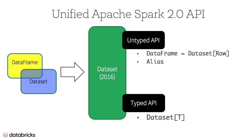
Diagram of the Unified Dataset API in Apache Spark 2.0
 

Datasets

 
Starting in Spark 2.0, Dataset takes on two distinct APIs characteristics: a strongly-typedAPI and an untyped API, as shown in the table below. Conceptually, consider DataFrame as an alias for a collection of generic objects Dataset[Row], where a Row is a generic untypedJVM object. Dataset, by contrast, is a collection of strongly-typed JVM objects, dictated by a case class you define in Scala or a class in Java.
 

Typed and Un-typed APIs
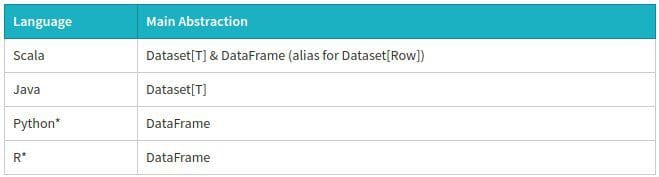
 

Abstraction types
Note: Since Python and R have no compile-time type-safety, we only have untyped APIs, namely DataFrames.


Benefits of Dataset APIs

 
As a Spark developer, you benefit with the DataFrame and Dataset unified APIs in Spark 2.0 in a number of ways.
 

1. Static-typing and runtime type-safety

 
Consider static-typing and runtime safety as a spectrum, with SQL least restrictive to Dataset most restrictive. For instance, in your Spark SQL string queries, you won’t know a syntax error until runtime (which could be costly), whereas in DataFrames and Datasets you can catch errors at compile time (which saves developer-time and costs). That is, if you invoke a function in DataFrame that is not part of the API, the compiler will catch it. However, it won’t detect a non-existing column name until runtime.

At the far end of the spectrum is Dataset, most restrictive. Since Dataset APIs are all expressed as lambda functions and JVM typed objects, any mismatch of typed-parameters will be detected at compile time. Also, your analysis error can be detected at compile time too, when using Datasets, hence saving developer-time and costs.

All this translates to is a spectrum of type-safety along syntax and analysis error in your Spark code, with Datasets as most restrictive yet productive for a developer.
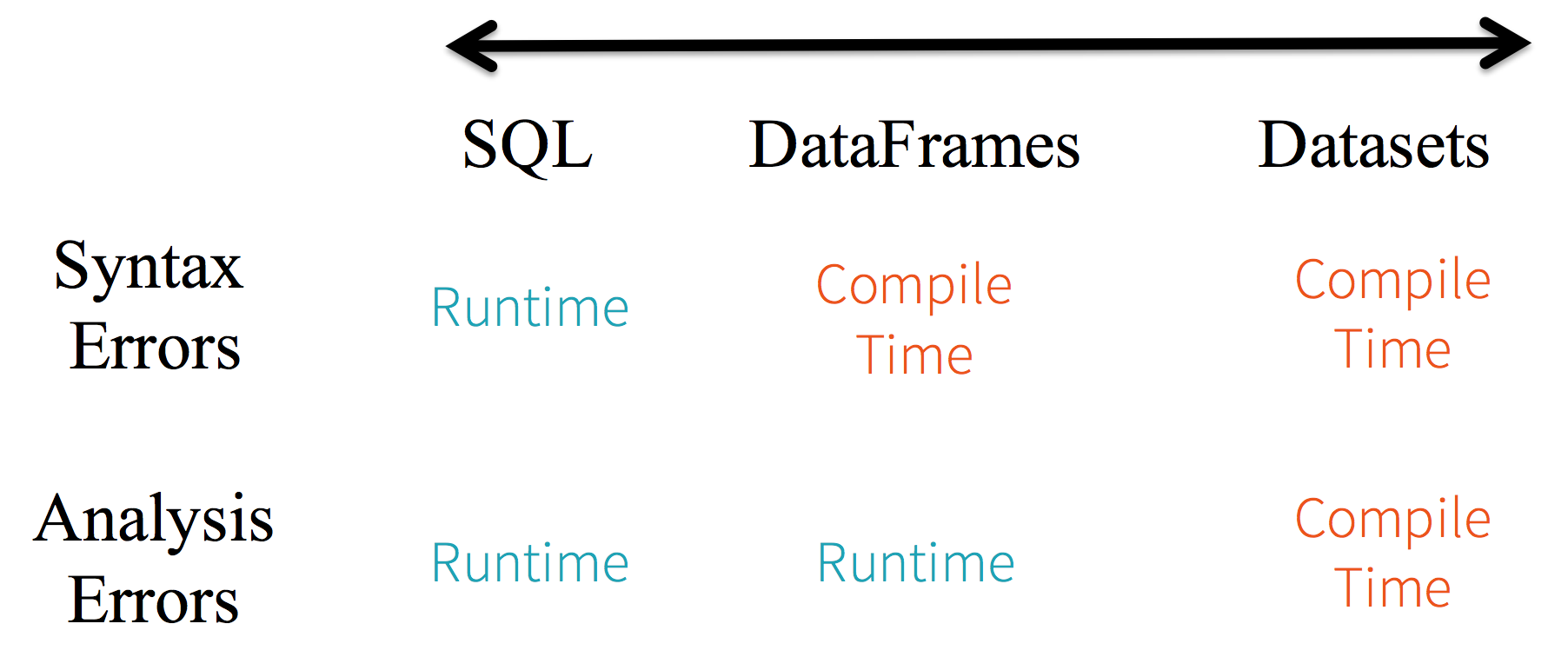
Type-safety spectrum between SQL, DataFrames and Datasets
 

2. High-level abstraction and custom view into structured and semi-structured data

 
DataFrames as a collection of Datasets[Row] render a structured custom view into your semi-structured data. For instance, let’s say, you have a huge IoT device event dataset, expressed as JSON. Since JSON is a semi-structured format, it lends itself well to employing Dataset as a collection of strongly typed-specific Dataset[DeviceIoTData].

{"device_id": 198164, "device_name": "sensor-pad-198164owomcJZ", "ip": "80.55.20.25", "cca2": "PL", "cca3": "POL", "cn": "Poland", "latitude": 53.080000, "longitude": 18.620000, "scale": "Celsius", "temp": 21, "humidity": 65, "battery_level": 8, "c02_level": 1408, "lcd": "red", "timestamp" :1458081226051}


You could express each JSON entry as DeviceIoTData, a custom object, with a Scala case class.

case class DeviceIoTData (battery_level: Long, c02_level: Long, cca2: String, cca3: String, cn: String, device_id: Long, device_name: String, humidity: Long, ip: String, latitude: Double, lcd: String, longitude: Double, scale:String, temp: Long, timestamp: Long)


Next, we can read the data from a JSON file.

// read the json file and create the dataset from the 
// case class DeviceIoTData
// ds is now a collection of JVM Scala objects DeviceIoTData
val ds = spark.read.json(“/databricks-public-datasets/data/iot/iot_devices.json”).as[DeviceIoTData]


Three things happen here under the hood in the code above:

  1. Spark reads the JSON, infers the schema, and creates a collection of DataFrames.
  2. At this point, Spark converts your data into DataFrame = Dataset[Row], a collection of generic Row object, since it does not know the exact type.
  3. Now, Spark converts the Dataset[Row] -> Dataset[DeviceIoTData] type-specific Scala JVM object, as dictated by the class DeviceIoTData.

Most of us have who work with structured data are accustomed to viewing and processing data in either columnar manner or accessing specific attributes within an object. With Dataset as a collection of Dataset[ElementType] typed objects, you seamlessly get both compile-time safety and custom view for strongly-typed JVM objects. And your resulting strongly-typed Dataset[T] from above code can be easily displayed or processed with high-level methods.
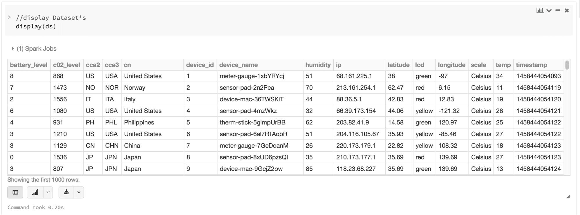
Screenshot of a table visualization of a Dataset in Databricks
 

3. Ease-of-use of APIs with structure

 
Although structure may limit control in what your Spark program can do with data, it introduces rich semantics and an easy set of domain specific operations that can be expressed as high-level constructs. Most computations, however, can be accomplished with Dataset’s high-level APIs. For example, it’s much simpler to perform aggselectsumavgmapfilter, or groupBy operations by accessing a Dataset typed object’s DeviceIoTData than using RDD rows’ data fields.

Expressing your computation in a domain specific API is far simpler and easier than with relation algebra type expressions (in RDDs). For instance, the code below will filter() and  map() create another immutable Dataset.

// Use filter(), map(), groupBy() country, and compute avg() 
// for temperatures and humidity. This operation results in 
// another immutable Dataset. The query is simpler to read, 
// and expressive

val dsAvgTmp = ds.filter(d => {d.temp > 25}).map(d => (d.temp, d.humidity, d.cca3)).groupBy($"_3").avg()

//display the resulting dataset
display(dsAvgTmp)
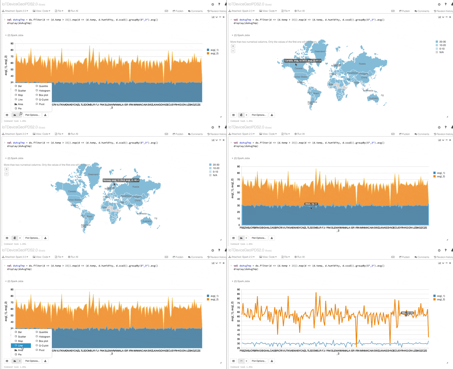

Example of visualizing a Dataset in Databricks
 

4. Performance and Optimization

 
Along with all the above benefits, you cannot overlook the space efficiency and performance gains in using DataFrames and Dataset APIs for two reasons.

First, because DataFrame and Dataset APIs are built on top of the Spark SQL engine, it uses Catalyst to generate an optimized logical and physical query plan. Across R, Java, Scala, or Python DataFrame/Dataset APIs, all relation type queries undergo the same code optimizer, providing the space and speed efficiency. Whereas the Dataset[T] typed API is optimized for data engineering tasks, the untyped Dataset[Row] (an alias of DataFrame) is even faster and suitable for interactive analysis.
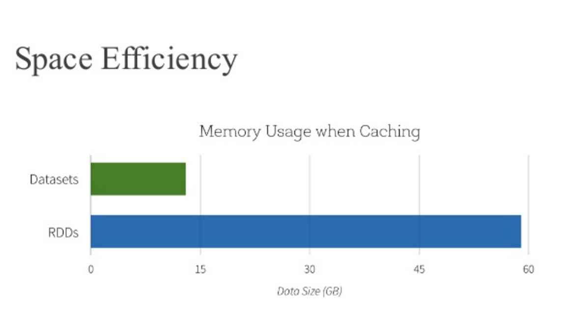
Datasets are much more memory efficient than RDDs

Second, since Spark as a compiler understands your Dataset type JVM object, it maps your type-specific JVM object to Tungsten’s internal memory representation using Encoders. As a result, Tungsten Encoders can efficiently serialize/deserialize JVM objects as well as generate compact bytecode that can execute at superior speeds.


When should I use DataFrames or Datasets?

  • If you want rich semantics, high-level abstractions, and domain specific APIs, use DataFrame or Dataset.
  • If your processing demands high-level expressions, filters, maps, aggregation, averages, sum, SQL queries, columnar access and use of lambda functions on semi-structured data, use DataFrame or Dataset.
  • If you want higher degree of type-safety at compile time, want typed JVM objects, take advantage of Catalyst optimization, and benefit from Tungsten’s efficient code generation, use Dataset.
  • If you want unification and simplification of APIs across Spark Libraries, use DataFrame or Dataset.
  • If you are a R user, use DataFrames.
  • If you are a Python user, use DataFrames and resort back to RDDs if you need more control.

Note that you can always seamlessly interoperate or convert from DataFrame and/or Dataset to an RDD, by simple method call .rdd. For instance,

// select specific fields from the Dataset, apply a predicate
// using the where() method, convert to an RDD, and show first 10
// RDD rows
val deviceEventsDS = ds.select($"device_name", $"cca3", $"c02_level").where($"c02_level" > 1300)
// convert to RDDs and take the first 10 rows
val eventsRDD = deviceEventsDS.rdd.take(10)
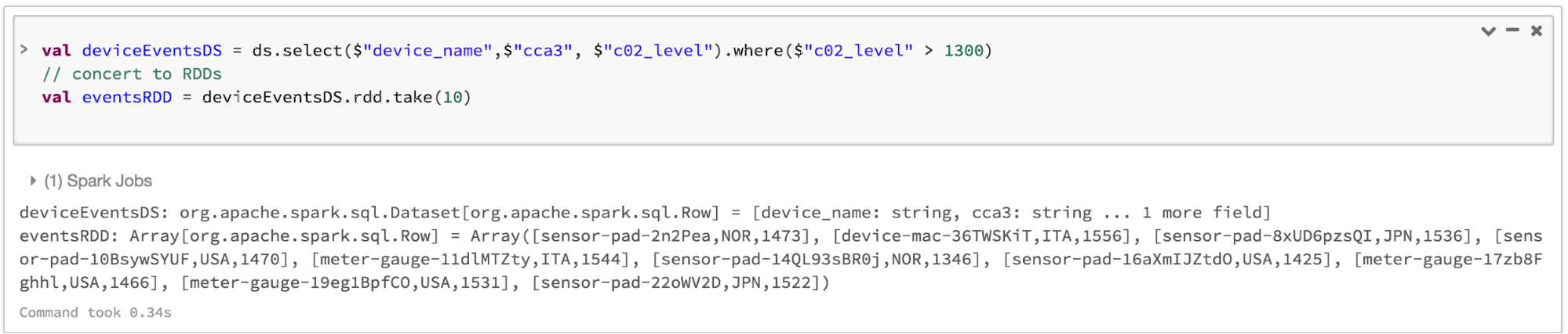

Screenshot of Spark converting a Dataset to an RDD on Databricks
 

Bringing It All Together

 
In summation, the choice of when to use RDD or DataFrame and/or Dataset seems obvious. While the former offers you low-level functionality and control, the latter allows custom view and structure, offers high-level and domain specific operations, saves space, and executes at superior speeds.

As we examined the lessons we learned from early releases of Spark—how to simplify Spark for developers, how to optimize and make it performant—we decided to elevate the low-level RDD APIs to a high-level abstraction as DataFrame and Dataset and to build this unified data abstraction across  libraries atop Catalyst optimizer and Tungsten.

Pick one—DataFrames and/or Dataset or RDDs APIs—that meets your needs and use-case, but I would not be surprised if you fall into the camp of most developers who work with structure and semi-structured data.